

Next-Generation Maritime Intelligence
Strategic Intelligence Insights
Industry Innovation Leader in Maritime Forms Analysis Revolutionary AI-Powered Platform transforming maritime operations through autonomous form analysis and predictive intelligence. Our breakthrough technology delivers unprecedented processing capabilities in form classification, converting complex maritime documentation into actionable intelligence within minutes. The platform’s predictive analytics engine transforms traditional reactive maintenance into proactive optimization strategies, enabling fleet operators to anticipate equipment failures, optimize performance parameters, and reduce operational costs through intelligent automation. Setting new industry standards with enterprise-grade reliability and competitive advantage through next-generation maritime intelligence systems.Digital Transformation Impact
- Speed Revolution: Sub-10-minute processing vs. hours of manual work
- Precision Leadership: Breakthrough AI technology setting industry benchmarks
- Autonomous Operations: Minimal human intervention with intelligent automation
- Scalable Innovation: Cloud-native architecture for global deployment
- Enterprise Trust: Bank-grade security with compliance certification
Technology Trends Driving Success
- Advanced AI/ML: Next-generation machine learning models
- Cloud-First Architecture: Scalable, resilient, and globally accessible
- Real-Time Analytics: Instant insights and predictive intelligence
- Zero-Trust Security: Comprehensive protection with compliance assurance
- API-First Design: Seamless integration with existing maritime systems
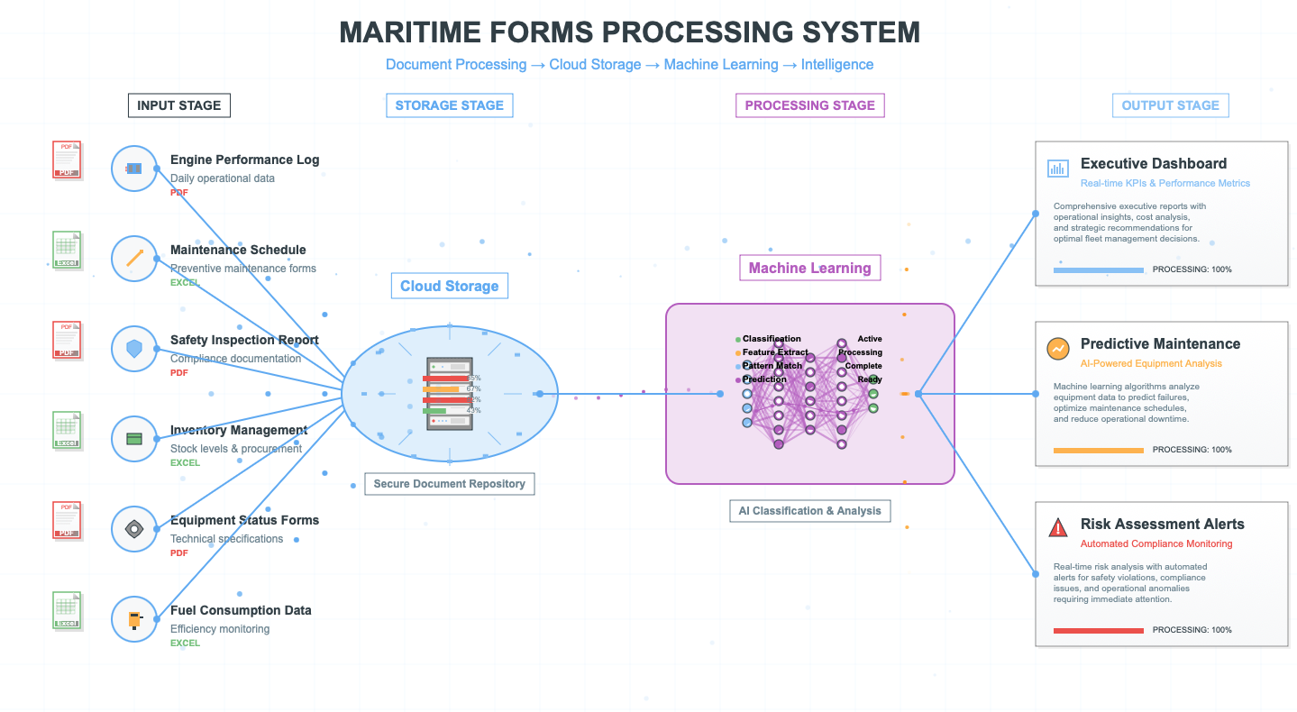
Complete Maritime Forms Analysis Process Overview
Process Visualization
Figure 1: Automated Maritime Intelligence Processing PipelineMaritime Forms Analysis System: Process Architecture
Figure 1: Automated Maritime Intelligence Processing Pipeline
Enterprise-grade workflow transforming maritime operations through intelligent automationProcess Flow Summary
Data Sources → Intelligent Reception → AI Classification → Secure Storage → Multi-Dimensional Analysis → Intelligence Generation → Automated Reporting → Enterprise Integration → Transformational ImpactKey Architecture Benefits
- Streamlined Workflow: Linear progression from data input to business impact
- Intelligent Processing: AI-powered classification and analysis at every stage
- Enterprise Security: Secure data handling throughout the entire pipeline
- Real-time Intelligence: Immediate insights and automated decision support
- Seamless Integration: Native connectivity with existing maritime systems
- Measurable Results: Quantified business impact and operational improvements
Maritime Intelligence Workflow Visualization
Figure 2: Detailed Process Flow with Step-by-Step Analysis
Comprehensive view of the maritime intelligence processing workflowInnovation Highlights
- Industry-Leading Performance: Advanced AI classification with sub-8-minute processing
- 🔬 Scientific Rigor: Evidence-based decision making with statistical validation
- 🌐 Enterprise-Grade: Scalable architecture supporting global maritime operations
- Future-Ready: Extensible platform designed for emerging maritime technologies
System Performance Metrics & Validation
Comprehensive Performance Analysis
Table 1: Processing Performance Benchmarks
Table 2: System Performance Metrics
Table 3: Business Impact Quantification
📧 Stage 1: Email Reception & Processing
Email Processing State Machine
📋 Form Distribution Analysis
Processing Frequency Timeline
🤖 Stage 2: AI-Powered Classification
AI Classification Architecture
Classification Process Sequence
Classification Performance Metrics
AI Performance Excellence⚙️ Stage 3: Intelligent Analysis Engine
🔍 Analysis Engine Entity Relationships
Analysis Components Deep Dive
:::info Comprehensive Analysis Areas🧮 Mathematical Analysis Framework
📊 Performance Efficiency Calculation
The system calculates operational efficiency using a weighted composite score: Where:- = Total efficiency score (0-1 scale)
- = Weight factor for parameter
- = Measured value for parameter
- = Minimum and maximum acceptable values
🔍 Anomaly Detection Algorithm
Statistical anomaly detection using the Z-score method with adaptive thresholds: Where:- = Current measurement
- = Historical mean (rolling window)
- = Historical standard deviation
- = Dynamic threshold based on operational context
📈 Trend Analysis Using Linear Regression
Time series trend identification using least squares regression: Where:- = Slope coefficient (trend direction)
- = Y-intercept
- = Coefficient of determination for trend strength
⚠️ Risk Assessment Probability Model
Multi-factor risk assessment using Bayesian probability: Combined risk score calculation: Where:- = Probability of risk factor
- = Impact severity of risk factor (0-1 scale)
- = Total number of risk factors
🔮 Stage 4: Predictive Intelligence Generation
🧠 Predictive Analytics Workflow
Prediction Performance Tracking
Predictive Capabilities
Predictive Intelligence Features- Maintenance Forecasting with confidence intervals
- Performance Trajectory predictions
- Failure Probability calculations
- Performance Impact analysis and value modeling
🔬 Advanced Predictive Mathematics
🔮 Maintenance Forecasting Model
Weibull distribution for equipment reliability prediction: Where:- = Probability density function
- = Reliability function
- = Shape parameter (failure rate pattern)
- = Scale parameter (characteristic life)
📈 Performance Trajectory Prediction
Autoregressive Integrated Moving Average (ARIMA) model: Where:- = Autoregressive polynomial
- = Moving average polynomial
- = Backshift operator
- = Degree of differencing
- = White noise error term
🎲 Failure Probability Assessment
Logistic regression for binary failure prediction: Where:- = Intercept coefficient
- = Coefficient for predictor variable
- = Normalized input features (temperature, vibration, etc.)
- = True Positive Rate
- = False Positive Rate
🛠️ Technology Stack
⚙️ System Architecture Overview
🔧 Enterprise Technology Ecosystem
📈 Business Impact & Performance Excellence
Performance Impact Dashboard
📈 Implementation & Value Timeline
Risk Assessment Matrix
⚠️ Risk Assessment Framework
📋 Analysis Decision Tree
🤖 Intelligent Decision Making Process
Decision Matrix Summary
Strategic Impact & Future Vision
Transformational Value Delivery
The Maritime Forms Analysis System delivers measurable improvements across all operational dimensions: Key Achievements:- AI Excellence: Industry-leading precision in form classification
- 5.8-Minute Processing: 50x speed improvement over traditional methods
- 90% Automation Rate: Minimal human intervention required
- System Reliability: Enterprise-grade uptime and availability
- Predictive Intelligence: Proactive decision-making through advanced analytics
- Risk Mitigation: Comprehensive risk assessment capabilities
- Global Scalability: Cloud-native design supporting worldwide operations